Today I am writing about a sketch for an idea I am working on implementing and will present in an extended form before the New Year, when I have time to write during the holidays. I enjoy toying with cellular automata. What appeals about the cellular autamata model is that it is perfect for exploring abstract models of emergence. Whatever side of the fence you sit when it comes to reductionism verus holism, you can’t deny the beauty in a propagating wave sustained through no abitrator.

A portion of my research involves working with mass-spring networks for model locomotion dynamics. During one particulary quiet lunch, I toyed around with the idea of combining a cellular automta lattice model with a mass-spring network model. The two, it turns out, complement quite nicely, as both are mediated by local interactions. In this mass-spring cellular automata (MSCA), a cell is represented by a point mass and the mass is equal for all cells. For a simple Von Neumann neighbourhood each cell is connected to four other cells via eight springs - two springs for connecting each neighbour to the centre cell. Why two springs? It should become clear soon. A spring has a single parameter which is its target length $\hat{L}$, a constant $k$ denoting the speed at which all springs move towards their target, and $L(t)$ denoting the current length of the spring at time $t$. The equation of motion for a spring is:

$\frac{dL}{dt} = k(\hat{L} - L)$

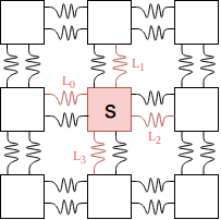
Each cell can control four of the springs connected to it, but adjusting the target lengths. Therefore the distance between any two cells, after enough time for the oscillations to have settled, will be the average of the two cells target lengths for their springs connecting one another. The model from the perspective of one cell is shown below.

Now here is where many variations of this model can be devised. For this journal entry I will discuss one; for the post at the end of this month I will explore more. Each cell also has a state $0 \leq s \leq 1$, which represents the coefficient of friction of that cell’s mass against the floor. Without different friction properties of the cell masses, the system would be unable to move its centre of mass. We define each cell’s state and its four spring length targets as a function of its neighbours’ states

$<s,\hat{L}_0,\hat{L}_1,\hat{L}_2,\hat{L}_3> = f(n(s))$

where $n(s)$ is the set of states of the neighbours of cell $s$. because the state of the cell is now represented by a five-dimensional continuous-valued vector, the function is more complicated than a traditional discrete cellular automata. To simplify, we discretise:

$s \in {0,1}$

$L \in {H, D}$

Where $H$ and $D$ are constants for the largest and smallest spring lengths allowed. I chose two settings to keep the model simple. The values for $s$ allow a mass to either be sticky or be frictionless, and the values for the springs allow for close or far connections. How many possible rules are there? Well the number of possible inputs to the function is $2^4$, but if a cell also references its own state then $2^5$. The number of possible outputs is $2^5$. So therefore the number of possible rules mapping between the inputs and outputs is $(2^5)^{(2^5)}$ or $2^{160}$. It might make more sense to adapt the function to a function of the link targets, for the reason that these represent the choices the neighbouring cells make better than a neighbouring cell’s state. This would give us ${(2^5)}^{(2^4)}$ possible rules. A meagre reduction.

What is exciting about the MSCA is that the cells and the lattice are dynamic. I imagine some interesting movements, clustering, and wave behaviours will develop. Another aspect I am thinking about is how to adjust the topology as the system evolves, so that cells can break away from neighbours and form groups. More to come this month!