
In a previous post I alluded to the curiously-named Movable Feast Machine. This blog post will elaborate on the movable feast machine and, through a small tutorial, guide you through a new computing paradigm. A paradigm that I find especially alluring because the problem solving techniques to write software for it are so orthogonal to our current standards. First, I will introduce you to Dave Ackley’s Movable Feast Machine $($or MFM$)$, a device designed to operate with the new computing technique. I will summarise Dave’s thoughts on the machine, describe my own ruminations about it, and point you to some further resources to help you continue exploring. Second, in the importance of avoiding too much theory and instead surfacing our inner Galileo or Brunel engineers, I will step through writing the code for and executing a program for the Movable Feast Machine. Dave has provided a few tutorials online, accompanied with example projects in the MFM code base - please take a look at these in conjunction with this post. My goal is to contribute to the momentum which Dave has begun by adding just one drop to the pool of resources to help others understand this young computing paradigm. This post will teach you how to develop a process for the MFM by building a Voronoi diagram using the ‘Best Effort Voronoi’ algorithm, or BEV for short. To realise the BEV algorithm took a few months of frustration, fear, and fantasising, but I am pleased by the final results. My experience designing the BEV algorithm has led me to believe that the software developer of the future may have a skill set resembling in silico chemists instead of the for-loop-fanatics in today’s world.
The Last Supper
In some future post I plan to write a comprehensive and historical analysis of the best effort computing paradigm. But, to climatise you to the new thought process required to design MFM algorithms, I will begin with but a brief background on the paradigm. Best effort computing is the dual to the widespread deterministic computing standard. In best effort computing the computer tries its best to produce the right answer; that answer may only be close to the true answer. Of course in deterministic computing, a computer can emulate non-determinism using ‘probabilities’ (I quote them because they are not true probabilities), which can reduce computation for intractable problems and give an accurate output within some probability margin. There are many fast algorithms that use this technique. Although similar in concept, best effort is different from a probabilistic algorithm built on a deterministic framework. To understand why, we need step backwards to a higher level. Best effort is a by-product of a larger computing paradigm called robust computing. In the land of robustness, the focus is on system security, hence optimality must be sacrificed. The computer architecture is not discretised into a bloated RAM farm and a single CPU that bottlenecks the information processing as is the case in modern computers, but instead the architecture is distributed into decentralised units where each unit has a small piece of coupled processing and memory power. Picture a neuron cluster where each neuron has a memory-forming synapse and a computing soma. Some may assert that this design patterns smells of distributed computing, and to some degree it does. But robust computing appears to cause phase transitions in the behaviour of the system as the number of simple processing-memory units grows large, whereas distributed computing is bounded in scalability and hence may never reach the critical masses for important phase transitions. Dave Ackley, the conceiver of the the best effort and robust computing paradigms, envisions a future where handfuls of computing matter can be scooped from your radio to patch a hole in your TV while both devices process. A scene which surely tickles the sci-fi fanatic within any futurist. This patching of hardware while devices continue computing is termed indefinite scalability. An uncanny likeness between these computers and you and I is apparent the more one dwells on this computing approach. Our cells $($and our alien cells, such as bacteria$)$ perform their tasks without global arbitration. At times, some of our cells fail, perhaps by failing to make a vital protein in time to stave a foreign virus, but the system - our body - maintains almost a homeostatic bliss. A rhythmic hum as we perform our daily doings. Cuts, infections, and illnesses are violently eradicated, and yet we nonchalantly paw through a book or write a letter.
In the context of best effort computing, Dave has coined the term, Correctness-Cost Curve: the cost to get a certain amount of correctness in the output of a best effort computer. Medical machines, construction vehicles, and space travel require high correctness and therefore will demand higher costs. But, a caretaking robot may require less correctness. The robot could miss a few instructions or clean the kitchen incorrectly, but the repercussions of its errors are far less ruinous. Think of how the human anatomy has some components which must function flawlessly to prevent catastrophic failure, and other components which fail hourly. Why did we not evolve twelve hearts? Because we can pay the cost for highly reliable ‘heart hardware’. A great span of the vascular system is redundant and damage or failure in these redundant places does not demand immediate recovery. We do not pay the expense for reliable ‘vascular hardware’ in the entire system.
Can this hectic computation be imbued into silicon? Perhaps not. But, robust and best effort computing are steps towards a new computing future. In the future, I see myself heavily adapting my research and personal projects towards promoting the best effort computing paradigm. This post is one in a series of posts whose objective is to start developing some literature on this subject. I am unsure whether my grasp of this new field will ever be as clear as my vision for it. If you are interested in more information on this computing paradigm please take a look at Dave Ackley’s recent research papers and lectures. Specifically I recommend the new T2 Tile Project, where a silicon computer archiecture is in live development, and this video about the motivation and theory behind the principles, where Dave rebuttals well many scepticisms about the paradigm. I see robust computing as humanity’s technological transition to multi-cellularity. Some time after the first billion years of evolutionary history, multi-cellularity became more economic than trying to increase the upper bound on a cell’s maximum size. Instead, cell’s remained smaller but stacked together into domineering blobs like the Grex. Similarly, computing trends appear to be approaching a computation ceiling and a useful growth in the number of transistors is either not possible or not economical. To force more computation inside a machine, we may have to forge a new path: decrease the burden of computation that any one machine performs and, alternatively, allow machines to become task-specific experts. A heterogeneous conglomeration of these specialist computers would quench this looming computational drought.
Best effort computing algorithms are referred to as processes because the line between initiation and termination of the usual algorithm is hazy (where does the algorithm for making ‘you’ start and end?). A process continues performing its intended task in the best way it can until either an adversarial process consumes it or the process seamlessly blends into a new process. Hence processes should be described as evolving rather than ending or beginning. In this post we will write the code for a process that creates Voronoi diagrams in the Movable Feast Machine simulator.
What’s So Good About Voronoi?
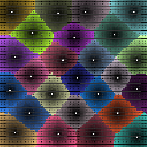
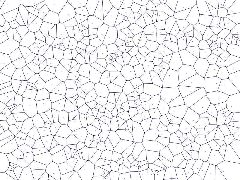
Before introducing the Best Effort Voronoi algorithm, I want to motivate it by exploring why Voronoi diagrams are useful. In compiling a list of uses, there are certainly applications of Voronoi tessellations which I have overlooked, please feel free to accumulate these in the comments below. If your eagerness for knowing BEV overrides your curiosity of its application, then feel free to jab the page down button and scoot along. For those who are unfamiliar with Voronoi diagrams, you have certainly encountered one before, but not under the Voronoi guise. Simply, a Voronoi diagram is a tiling of a space which divides up the space around a scattering of central points so that each point in the space is assigned to a region according to which central point it is closest to. Take a look at this example borrowed from here.
Voronoi diagrams are abundant in nature. As with most mathematical abstractions, the Voronois we find in nature are imperfections of their divine geometrical brethren. But physics gave birth to biology and physics is optimal, thus the trend towards optimal Voronois is inherent in the nature of living things. Bumblebees, for example, economise their use of wax by minimising the distance between the positions of the honeycomb cells, resulting in a homogeneous tiling of the honeycomb. This innate behaviour produces a symmetrical Voronoi - perfection at two levels.

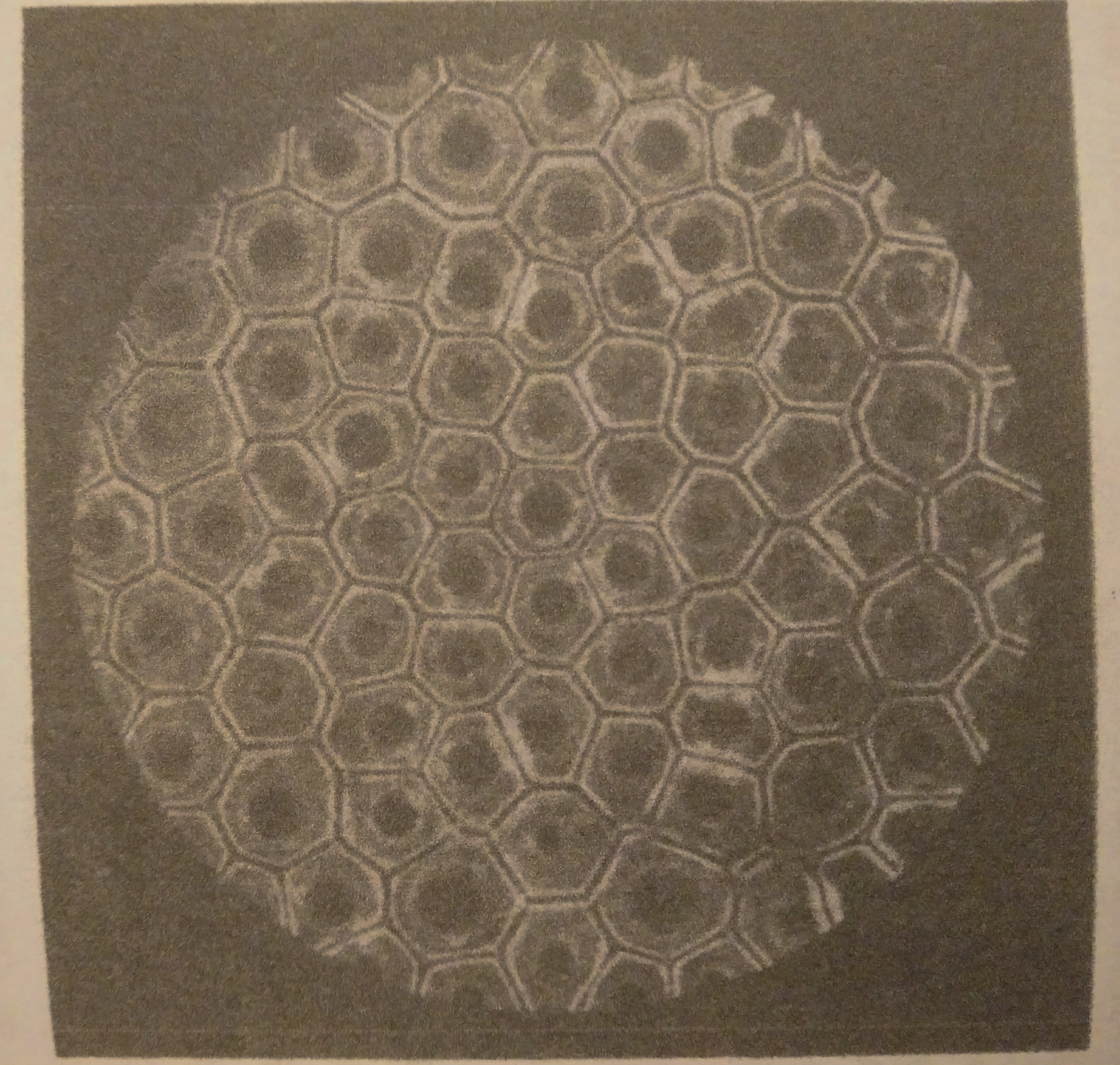
The word ‘Voronoi’ usually appears in the same context as the word ‘cell’. Peering through a microscope at some animal tissue will present another Voronoi cell pairing. Here the multicellular mass has organised itself such that each cell’s membrane is equidistant from any two neighbour pairs’ nuclei. Although this organisation may seem obvious, take care to understand that it is the property of the cell that produces this outcome. The cell tissue Voronoi is a decentralised work of art. Could cells exist that cannot produce Voronoi diagrams? Yes. D’Arcy Thompson showed us in On Growth and Form that cells seek to minimise their surface area and in ideal conditions will tessellate in a manner true to Voronoi, but this process can have its imperfections. Like how the building of crystals results in defects because of the disorganised assembly process.
Another favourite natural Voronoi of mine is bubbles. Bubbles and cells share many similar properties, so the basis for the cells’ inclination to make Voronoi diagrams may be inherited from its bubble origin. Bubbles tessellate a plane due to how water behaves: it seeks to minimise its surface energy, causing bubbles on the surface to be pulled together by the presence of meniscuses. I will not include a photo of the bubble Voronoi so as to encourage you to seek out this phenomenon in reality.
Now that it is established that Voronoi’s exist at many scales of life, how can we exploit this pattern for solving problems? To begin, let’s discuss the information which can be obtained from a Voronoi diagram. The honeycomb cell, tissue cell, and bubbles are all examples where some optimality is reached. Given some fixed set of cell foci, a Voronoi tessellation is the optimum boundary placement such that each cell has the maximum amount of area within its boundary. Huh. Also, the boundary between any two cell foci is equidistant, so if an object were to be placed on one side of the boundary rather than the other, that object must be positioned closer to the cell’s foci whose side of the boundary the object is on. A classification system of this kind is called 1-Nearest Neighbours. If each of the cell foci represented a data point, for example its two-dimensional position might represented height and age of an individual, and the cell was coloured according to the gender of that individual $($red for male, green for female$)$, then if a new data point was placed on the diagram whose gender was unknown, a valid prediction might be to classify it according to the data point it is most near. Or, in other words, classify it by whichever Voronoi cell encloses the data point. This approach has some limitations of which there is not space to discuss, but the scheme is interesting nonetheless. Another application for Voronoi diagrams is Vector Quantisation, an algorithm for reducing the dimensionality of a space by identifying each part of the space by its cell index. Thus an $N$-dimensional space can be reduced to a 1-dimensional Voronoi space. These two examples are data processing applications for Voronoi diagrams, but rest assured that a Voronoi diagram is a transdisciplinary tool. Here is a use of a Voronoi diagram to tessellate a map of schools in Melbourne so that parent’s know the nearest school for their child to go to. Take a look at the Wikipedia page for over twenty-five ways that Voronoi diagrams are used.
Best Effort Voronoi
Now that the importance of Voronoi diagrams has been stressed, the rest of this post will discuss the design and implementation of the Best Effort Voronoi (BEV) algorithm for creating robust Voronoi diagrams on the Movable Feast Machine. When designing the BEV algorithm there were three properties I believed it required to be robust:
-
) Decentralised Formation: the traditional Voronoi diagram is a spray of points in a space, where some geometry and linear algebra is used to compute midpoint lines between all points which are then used to calculate perpendicular lines from these midpoints. The boundary lines are then connected with ray intersection. The naive algorithm to generate a Voronoi diagram is $O(n^2)$. There are interesting heuristics and optimisations that the research community has invented, but these will not be covered here. The problem with these approaches is that they do not align with the mantras of robust-first computing outlined earlier. For example, if the point count is in the billions instead of the hundreds, any algorithm on a single computer will struggle. To manage such a tsunami of points, we could distribute our point quantity across multiple computers and have these computers communicate between one another accurately $($and efficiently$)$ to orchestrate a Voronoi diagram. This might seem a reasonable approach to deterministic thinkers of today, but real life applications show how quickly it can become useless. Say each point is associated to one computer. That’s impractical you say! Well say each of those points was a house, or a human, and we wanted to compute a Voronoi diagram of the Earth. Before the twenty-first century, few would have had the compute power for such a task. Now a modern cloud cluster might scale to handle the task over a month. But that’s just one computation assuming you have the GPS data for all the house locations correct, to mention one point of failure. But property development is a dynamical systems and it changes and evolves as fast as an E. Coli community in a petri of penicillin. Therefore we would need to rerun the $O(n^2)$, billion-point Voronoi algorithm each time the house distribution of the Earth changes, and be certain that satellite failures do not eradicate a Caribbean island from the diagram. This implies that the BEV algorithm must work in a system where many independent points are calculating Voronoi diagrams in parallel. The next two properties of the BEV algorithm branch from this first one.
-
) Addition and Subtraction of Points: Points should be able to be added and removed, and the BEV should adjust to these changes, but in a distributed, localised manner. Handling the case for removing points was the trickiest constraint and took me the longest to solve.
-
) Asynchrony: In the example of the houses as computing units that cooperate to tessellate the Earth, there a non-uniform distribution of resources. Some regions will have faster computing and their contribution to the diagram might complete before other regions. From the computer science algorithmist perspective this is a nightmare. Parallel threading, locks, or potentially centralised management of job allocation need to be considered. Creating this algorithm in the MFM world would increase the computation magnitude, but there is a subtle beauty to this because asynchrony is so much more robust and natural for real life problems.
With these conditions in mind, it is clear that implementing the BEV algorithm is a perfect opportunity to use the MFM system for a personal project; something I have been trying to garner the inspiration for. By using the MFM system we have already ‘satisfied’ properties (1) and (3) because they are innate to the system itself and therefore the BEV algorithm is helpless to incorporating them. This leaves property (3) unsatisfied. First I will describe the BEV algorithm and then explain how it satisfies property (3).
The BEV Algorithm
I cannot recall the reason why I posed myself the question of whether cellular automata can be used to create Voronoi diagrams. It is relatively unsurprising as I find myself constantly trying to map complex processes to simple cellular automata rules. A hallmark of complexity and ‘emergence’ $($Personally, I am not a fan of the word emergence and I avoid using it colloquially$)$. It is important to note that although I arrived at this algorithm myself, it is by no means entirely original work. After some paper rummaging I discovered similar algorithms have been invented before. The aspect of removing data points while the algorithm is running is original though, to the best of my knowledge.
To ease understanding, let’s begin with an analogy. Starting with a spattering of data points on a lattice, imagine each data point as an infinite water source which projects water molecules uniformly around it in all directions. Eight directions including diagonals, otherwise four. For a moment let’s look at one of these data points/water sources. The water molecules that have just been projected from this source will have maximum acceleration, but as they move on their trajectory away from the source they will collide with other air and water molecules that are moving slower, causing a transfer of energy away from the moving molecule and hence a drop in acceleration. Thus water molecules that are further from the source will be slower than those that are closer to the source, on average. We shall call this loss of energy a behaviour caused by friction in the simulation. The pressure of the water molecule is proportional to its acceleration, so instead of using the term acceleration, we will use the term pressure. The pressure decreases as the water moves from its source, but we aren’t concerned with whether this decrease in pressure is linearly related to the distance from the source because these details don’t affect the creation of the Voronoi diagram. Transforming this process into a cellular automata rule is relatively straight forward. Each cell will have a pressure value which represents its current pressure. For this to work on the MFM architecture this must be an integer due to the small memory constraints. Because we do not know how far we want our water to travel from its source, we cannot know what pressure value to assign the source cell because at some finite distance from the source a cell’s pressure will have to become negative. To ease our situation, let’s call the value ‘inverse-pressure’ instead and assign the source an inverse-pressure value of zero, or a pressure value of infinite. The rule for water movement is then as follows:
If any of your neighbour’s inverse-pressure values are lower than yours, assign your neighbour your inverse pressure value, plus one.
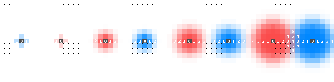
The best way to understand this rule is by example. First a diagram of the rule in action and then an explanation.
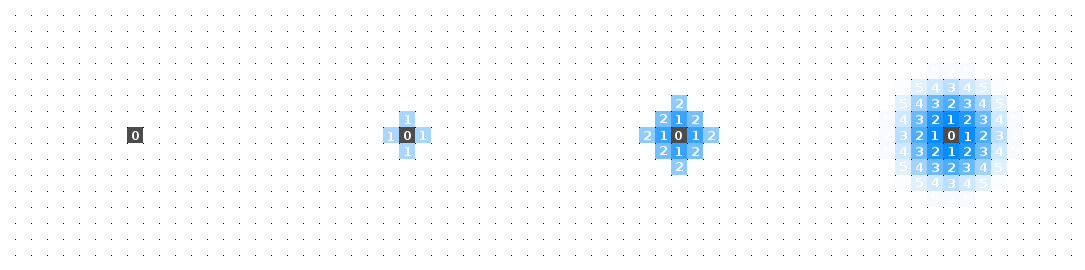
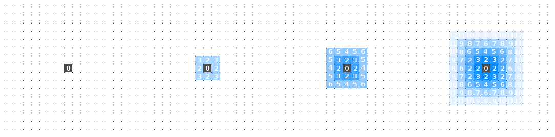
Frame (1) shows the source as the only cell on the lattice with any water, and as discussed, the inverse-pressure value of this water is zero. One time step and frame (2) shows that each of the north, south, east, and west neighbours - or Von Neumann neighbours - had no water, or an undetermined inverse-pressure which is assigned a value of zero, so their inverse-pressure values are updated to $0+1$ because they are larger than the source inverse-pressure. Frame (3) now performs this growth process for the five water-filled cells from frame (2). There is no change in the four newly filled cells from frame (2) because their inverse-pressure values were updated to $0+1$. Eight new cells have been added on the perimeter of the $1$ inverse pressure cells, this time with an inverse pressure of $1+1$. Frame (4) shows this process after a few time steps have soaked our lattice. Observe that we get a nice natural-number gradient converging on our source. Now let’s see how this process develops for two sources.
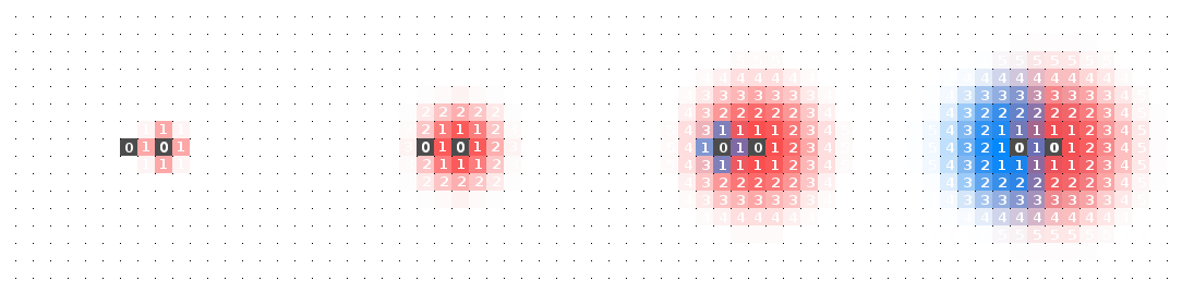
Interesting. Here we have shown only the inverse-pressure values for the lateral cells and some cells at the boundary. There is a point where our inverse-pressure gradient goes from positive to negative when moving between the two sources. By inspecting the location of this gradient we note that it is equidistant from both sources. “Voronoi!”, you might have exclaim upon the dawning of your realisation. This behaviour generalises when more sources are added. You might notice a distinctly sculpted look to the Voronoi diagrams that result. This can be smoothed by changing the neighbourhood of a cell to a Moore neighbourhood which includes diagonals. Now, water molecules that travel diagonally from the source are moving further than lateral moving molecules because of the properties of square lattices. To a close approximation the ratio of the diagonal distance travelled to the lateral distance travelled is $3:2$ $($the diagonal of a square is $\sqrt{2} \approx 1.41)$. A result of this adjustment is below.
Recall that property (3) of the BEV algorithm is that it must be asynchronous. This means that each of the cells should update and change the values of neighbouring cells in any order and at any time. On average all cells will update the same number of time steps within a timespan. Does the algorithm still work for the asynchronous scenario? Let’s see:
Yes! Why does it still work? Because there there are no race conditions in our algorithm. For example, even if one of the sources gets all the processing time and completely fills the area with its water, once the other source starts updating, its conditions only require that the inverse-pressure around it be higher for it to keep growing. Therefore once the system is run for long enough, a happy equilibrium develops. The result of this is that we have also satisfied half of property (2): data points can be added while the algorithm is running.
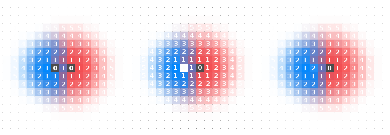
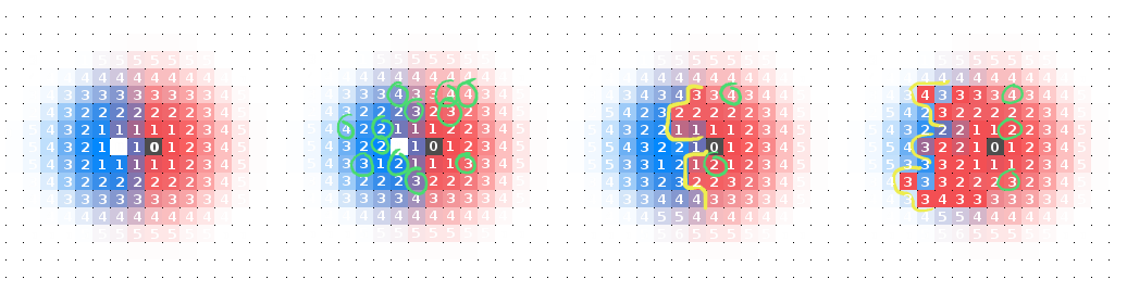
The Best Effort Voronoi algorithm so far has satisfied all the properties apart from the other half of property (2), which is the ability to remove data points. This requirement is not simple and a solution proved rather elusive. A few unsuccessful attempts were tried to solve this problem. A less elegant solution involved creating an ‘anti-source’ which absorbed all the water around it. But once I found the answer, I was delighted in both how simple and effective it was. I think the answer to this problem truly shows the power of best effort computing. Before I show you it, first take a look at the behaviour of the algorithm outlined when a source is removed. Try to see if you can complete the algorithm to solve source removal. It would be interesting if a different solution can be found other than the one I have used, yet equally elegant - or perhaps my solution is relatively simple after all and I unhesitantly submit to your asynchronous-algorithm greatness. Here is a diagram of why the BEV algorithm fails, without the correction for source removal:
Here’s my solution:
Every time step, increment a cell’s inverse-pressure value by one.
Either you smacked your forehead in disbelief or you guffawed at my naivety. Hindsight is twenty-twenty so please revel in how beautiful this solution is for a moment. Why does it work? Well first let’s check that the behaviour we had before has not changed with this addition. Here is a test for three sources, asynchronously running on the MFM simulator. The first video shows the algorithm without the new rule and the second video shows the algorithm with the new rule.
Video of two source cells running on the MFM without the +1 rule.
Video of two source cells running on the MFM with the +1 rule.
Other than a galactic flowing from the sources and a wobble of the dividing line between the three sources of the video with the new rule, the diagram is, to a close approximation, identical. The use of the term to a close approximation is crucial because it is a pillar of the best effort computing paradigm which was discussed at the start of this post. On average, the BEV algorithm will produce a Voronoi diagram, but the times when it produces an incorrect diagram, this incorrect diagram will have a small error margin. Potentially, the error could grow large if only a few sources processed for a while, but the probability of these errors collapses to near-zero as the number of points in the Voronoi diagram increases. Reflect on that for a moment and reread the section on best effort computing if needed.
Why does this solution solve the source removal problem? Let’s inspect the case for two sources as this will generalise to the case for any number of sources. There are two cases when this rule must work. First, when all sources are present, the rule must not hinder the creation of a Voronoi diagram. Second, when one or more sources is removed, the Voronoi diagram must adapt to now become a Voronoi diagram devoid of these removed sources. Let’s address the second point by slightly tweaking the process such that the new rule only applies when a source is removed and it only affects the cells which were from that source. This is not a realistic tweak because it would be complicated to implement in a decentralised system, but it helps for understanding. With this fictional algorithm, all the cells of the removed source continue incrementing their inverse-pressure value each time step. Some cells may update a little faster than others and may be consumed by their neighbours, but on average the entire population will increase. The cells at the boundaries will be the first destroyed because once their inverse-pressure values increment higher than any one of their conflicting neighbours’ values, the cells will be consumed. This consumption by neighbours will then continue until the centre of the removed point’s region where the final cell will be destroyed. Could the population fight back and reduce its inverse-pressure by some internal complex feedback? No. To do this would require the removed source because it can maintain a low inverse-pressure. With the source, any neighbours which started to grow dangerously large inverse-pressures around the source are corrected. This correction is then gradually propagated to cells at the boundary of the region, like a wave $($this is why the simulation shows galactic flowing behaviour from the source$)$. This wave does not move at the same rate uniformly because the system is asynchronous. But, over the average of all waves a region should remain relatively stable. The next diagram below should help make this clear.
Now reverting back to the BEV algorithm without its fictional correction we can also show why this rule still works even in the case where all sources are present and no one has been deleted. It is the opposite process that was mentioned for why a population without a source will eventually die. Throughout the entire Voronoi diagram, any cell could spontaneously increment and therefore risk destruction by one of its neighbours. But cells which perform this incrementation around a source will be corrected back to their original inverse-pressure by the source. Therefore cells which perform this incrementation around cells which are around a source will also eventually be corrected to their original inverse-pressure. By induction this rule applies to all cells in a region around a source and thus all cells will eventually be corrected to their original inverse-pressure and the Voronoi diagram will be preserved.
$($1$)$ Blue source cell is removed. $($2$)$ +1 perturbances of the inverse pressure of random cells $($in green$)$ do not affect the general diagram. $($3$)$ Perturbances in the blue cells cannot recover due to the missing source cell and a front of red cells $($in yellow$)$ begins to take over. $($4$)$ The red cells begin to take over until the blue cells are almost completely gone.
That concludes the algorithm. Wonderfully simple in its properties yet surprisingly organic in its result. Next, we will go through the process of writing the code to implement this algorithm yourself in the MFM system using the programming language Ulam.
BEV in Ulam
Before I begin, I encourage you to take a look at Dave and Elena Ackley’s paper introducing the Ulam programming language with some clean examples and intuitions behind the language’s design. This tutorial assumes knowledge of Ulam at the level of this paper.
Installing Ulam and MFM
$($NOTE: These instructions are performed on a machine running Ubuntu 14.04. I have not had the time to test this on other linux distributions or operating systems, but please feel free to comment if you have explored this.$)$
The Ulam language is used to write code which to compile and run on the Movable Feast Machine simulator. Therefore we need to install both Ulam and MFM to begin. I have used the instructions directly from the installation webpage which tell how to download and install from source. First, check you have the correct dependencies for everything to run. Update your package manager list.
$ sudo apt-get update
Install some dependencies.
$ sudo apt-get install git g++ libsdl1.2-dev libsdl-image1.2-dev libsdl-ttf2.0-dev libcrypt-openssl-bignum-perl libcrypt-openssl-rsa-perl libcapture-tiny-perl
If you don’t have git, install it.
$ sudo apt-get install git
You should have g++ if you are working through this from Ubuntu 14.04. If not install it.
$ sudo apt-get install g++
Now to install some more dependencies. For detailed descriptions of these please refer to the installation page. The following are for SDL support.
$ sudo apt-get install libsdl1.2-dev
$ sudo apt-get install libsdl-image1.2-dev
$ sudo apt-get install libsdl-ttf2.0-dev
And some Perl packages.
$ sudo apt-get install libcrypt-openssl-bignum-perl
$ sudo apt-get install libcrypt-openssl-rsa-perl
$ sudo apt-get install libcapture-tiny-perl
Now create a new directory to install both ULAM and MFM into. I called mine MfmWork/.
$ mkdir MfmWork
$ cd MfmWork
Clone the repositories for MFM and Ulam from git.
$ git clone https://github.com/DaveAckley/MFM
$ git clone https://github.com/DaveAckley/ULAM
Let’s install the MFM simulator first. Move into the directory of the repository.
$ cd MFM
And build.
$ make
If that works then the hardest part is behind you. If not, explore the installation page for debugging tips as I am afraid I do not have any to supply. Now move into the Ulam repository directory.
$ cd ../ULAM
And build.
$ make
$ make ulamexports
The installation page cautions that these builds could take some time. Go back and re-read the BEV algorithm while waiting. Once building is complete, let’s make sure the MFM simulator runs. First leave the ULAM directory and run the bash script in the MFM repository.
$ cd ..
$ ./MFM/bin/mfms
Enjoy the feast for a bit. Immediately you will get a window like this.
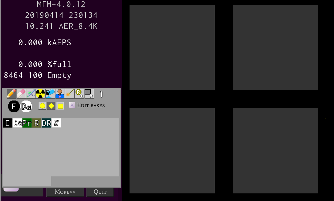
Your initial start-up layout might not look exactly as mine. Here are a few essentials to alleviate stressful simulator moments. ‘h’ toggles the purple help screen; ‘t’ toggles the white tool screen; hold Ctrl+Alt and drag either a window or the simulator view to move it around; select ‘atoms’ in the tool menu (grey floating box) and place them on the grey lattice and toggle ‘space bar’ to start and stop the simulation. Take a minute to explore these actions and discover anything else of value.
Software Skeleton
Create a new directory within ‘MfmWork’ titled ‘BevAlgorithm’.
$ mkdir BevAlgorithm
$ cd BevAlgorithm
Here is where you will create all the files and write all the Ulam code needed to compile and run the Best Effort Voronoi algorithm. There are three files to create. Create them and then I will explain each of their purposes.
$ touch Propagate.ulam
$ touch Propagator.ulam
$ touch Source.ulam
As with the majority of object-oriented programming languages $($ULAM is written in C++, which is object-oriented$)$, it is considered good standard to have one file per object to help keep the code manageable. Hence our three files represent three MFM objects. In the land of MFM there are two fundamental object types, Elements and Quarks. What about Hadrons? Not in MFM Universe I’m afraid. An Element is like a class in C-type languages, and a Quark is like to a virtual class. Suitably, instances of Elements are called Atoms.
- ) Propagate.ulam: This is the only Quark you will implement for this program. It describes the base methods for any Element which would like to spread out and compete with other propagating atoms.
- ) Source.ulam: This Element is the source or datatpoint, as mentioned during the description of the BEV algorithm. It inherits from the Propagate Quark because it needs to spread Atoms from its location. What’s special about the Source Element is that it cannot be deleted by other Propagators.
- ) Propagator.ulam: The spawn of the Source. This Element will continuously replicate to its neighbouring cells, but with increasing inverse-pressure. When two Propagators are neighbours they will try and consume each other. This Element inherits from the Propagate Quark.
Let’s start by making the Source Element. Because it inherits from the Propagate Quark this Element will not run as a standalone file, but it is the simplest of the three objects to implement and so it is an obvious choice for wetting the keyboard for some Ulam rapture.
Implementing the Source
Every basic Element in Ulam has the following anatomy $($an-atom-y?$)$:
\color #fff
\symbol Sy
\symmetries normal

element Adam : Qwark
{
    // type definitions
    // e.g. typedef Unsigned(4) Nibble;

    // parameter definitions
    // e.g. Nibble crumb;

    Void behave()
    {
        // Action!
    }
}
Let’s start with the pieces that are probably most familiar. The keyword element is like the class keyword in C++ and indicates that we are creating a new Element called Adam, in this example. Adam inherits from Qwark, which is a quark, but could also be an element. Inside the element definition we have three sections. The first section is for defining any type definitions. Each Atom object is treated as a self-contained unit which can perform its own computation via observing its neighbours to decide what to do next. Because future complex systems will require millions of these Atoms to interact $($think of how many cells are in your body$)$, each must have only a small amount of memory and computational power to easily be deployed and replicated. Each Atom is only given a small number of bits so memory conservation is important. No arbitrary int64 creations. The second section uses the type definitions from section one to create parameters within the element which are globally available. Nothing surprising here. The third section is a predefined method called behave which is argumentless and returnless. It acts as the main loop for the element, but unlike deterministic programming our loops are not guaranteed to execute sequentially and fairly. There could be hundreds of updates before an Atom is given the ability to run its behave snippet. What is important is that when the Atom does run its behave snippet, the system will become temporarily deterministic and allow the Atom to complete its process without interruption.
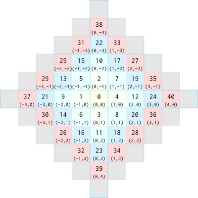
Now take a look at the top three lines of the skeleton file. Every element in the MFM must have a colour and symbol which distinguish it. Similar to how real elements can behave like one of 118 different elements in the periodic table, discounting isotopes. Really, the colour is for aesthetic purposes and only the symbol defines the element. On the third line we have the code \symmetries normal. This describes the element’s invariance to rotation. Some cellular automata, like Game of Life, are rotation invariant because the rules only involve the counts of neighbouring cells, while other rule sets incorporate positional properties of a cell’s neighbours. By setting the element symmetry to normal, any rules defined are not invariant, which means the west neighbour is always the same west neighbour. The symmetries could be set to all and thus our west neighbour is also our north, east, and south neighbour as the atom rule is rotated through all four of its symmetries. Refer to the Atom boundary diagram below if this is still confusing.
Using the definition outline above, we will create the Source Element. The Source Element will consist of two type definitions, one parameter, and three methods. Here’s the skeleton:
use Propagate

\color #fff
\symbol Sr
\symmetries normal

element Source : Propagate
{
    //TODO
}
Our Source Element inherits the as-yet-to-be-created Propagate Quark, is the colour white, has the unique symbol, ‘Sr’, and has no invariance for the rule matching. The first line tells us to import the Propagate Quark from the Propagate.ulam file. For the Voronoi diagram it would be useful if each cell had a colour corresponding to both its region and its inverse-pressure value. If all atoms were white, it would be difficult to persuade others of the effectiveness of the algorithm. To do this, assign each source a random colour when it is first created. This colour will then be assigned to the atoms it spawns. Create two type definitions like so:
typedef Unsigned(8) ColorValue;
typedef Unsigned(8) ARGB[4];
ColorValue is a 256-bit channel type, as anyone who has worked with graphics will be familiar with. ARGB just defines a four-element array of 256-bit elements, representing the programmer’s palette. Using the ARGB type, create a colour parameter for our Source Element:
ARGB col;
Next, we will create a method which is used only once when the Source Element is first initialised, and assigning it a random colour:
Void initSelf()
{
    Random rd;
    ColorValue r = (ColorValue)rd.between(30, 256);
    ColorValue g = (ColorValue)rd.between(30, 256);
    ColorValue b = (ColorValue)rd.between(30, 256);
    col[1] = r;
    col[2] = g;
    col[3] = b;
}
Random is a built-in class which allows us to sample from various discrete random distributions. Here we have chosen colour channel values between 30 and 256 and then assigned them to the RGB channel positions in the four-element ARGB colour array.
The Source Element will create a random colour upon creation, but that is the sum of its capabilities thus far. Time to wire in some behaviour. Our Source Element will interact with its eight neighbours and spawn Propagator Atoms in these locations. There are two scenarios for any atom that wishes to propagate to its neighbours: (1) The neighbouring cell is empty, or (2) The neighbouring cell already contains an atom. There will be two methods to handle each case just to make things clean. The two methods are inherited from the Propagate Quark, but first let’s implement them in the Source Element. There will be some redundancy in place of clarity because the Source Element’s response is the same whether the neighbouring cell is empty or occupied. Both methods will overwrite whatever is in the neighbouring cell with a Propagator Element that has some assigned inverse-pressure value. This also a reminder to give the Source Element a inverse-pressure parameter as well, which will be greater than all other inverse-pressure values. Add this line just before the Random rd; line in the initSelf method:
ip = 0;
‘ip’ stands for ‘inverse-pressure’. A type definition has not been made for this because it will be inherited from the Propagate Quark because all propagating atoms need an inverse pressure. Now let’s write code to spawn atoms around a Source Element. Create three methods:
Void emptySpace(Neighbour i)
{
    spawnPropagator(i);
}

Void captureSpace(Neighbour i)
{
    spawnPropagator(i);
}

Void spawnPropagator(Neighbour i)
{
    //TODO
}
As mentioned earlier, there is some redundancy in the first two methods, but it will make things easier when implementing the Propagator Element. All three methods take a Neighbour type which will be defined in the Propagate Quark and is just a five-bit unsigned integer to keep track of the neighbourhood. The following spawns a Propagator Atom at a neighbourhood index:
Void spawnPropagator(Neighbour i)
{
    Propagator p;
    ew[i] = (Atom)p;
}
The first line is simple enough and just creates a new Propagator Atom. The second line is less clear because we have this new term … ew? ew stands for EventWindow and is an array of atoms handled by the MFM simulator back-end. Each index of the EventWindow matches the atom neighbourhood diagram shown earlier and is a standard map for atom neighbour look up. If no atom exists at a particular index, a special atom called Empty is returned. To spawn the Propagator Atom at index i in the neighbourhood, it is as simple as casting the atom to a generic Atom element and updating the EventWindow value.
Looking at the atom neighbourhood diagram, indices one through nine constitute a Moore neighbourhood and indices one through five constitute a Von Neumann neighbourhood. Remember that diagonal neighbours are assigned an inverse-pressure $+3$ and lateral neighbours are assigned an inverse-pressure of $+2$ because the diagonals are slightly farther away. Let’s also assign the Propagator Atom that a Source Atom produces to match the colour of the source. The final code for the spawnPropagator method is:
Void spawnPropagator(Neighbour i)
{
    Propagator p;
    p.baseCol = col;
    if(i < 5) // if Moore neighbourhood
        p.ip = 2; // 0+2 = 2
    else
        p.ip = 3; // 0+3 = 3
    ew[i] = (Atom)p;
}
Well done. This completes the code for the Source Element. The code will not run until the Propagate Quark and the Propagator Element have been made. Onward.
Implementing the Propagate Quark
Now most of the quirks of the Ulam language have already been explained, I will start by providing the skeleton of the Propagate.ulam file.
quark Propagate
{
    typedef Unsigned(8) InvPressure;
    typedef Unsigned(5) Neighbourhood;

    EventWindow ew;
    InvPressure ip = 0;
    Once oc;

    virtual Void initSelf() {}
    virtual Void emptySpace(Neighbour i) {}
    virtual Void captureSpace(Neighbour i) {}

    Void behave()
    {
        //TODO
    }
}
The behave method is like the main method in a Java class, it is where all the class calls come through, when requested to execute.
Don’t sputter your tea in angst, the Once type isn’t too uneasy. It is essentially a boolean flag, that toggles the first time it is checked. This can be used as a clean way to call an initialisation in the behave, while being certain that an atom will only be initialised once. Add this code in the behave method to do just that:
if(oc.new())
    initSelf();
Some logic is required to iterate through the EventWindow and check if the neighbouring cells are empty or contain an atom. Recall the Von Neumann neighbourhood starts at index one and goes until index eight.
for(int i = 1; i < 9; ++i)
{
    Atom other = ew[i];
    if(other as Propagate)
        captureSpace(i);
    else if(other is Empty)
        emptySpace(i);
}
The first line in the for loop grabs an atom from the EventWindow - an empty space is an Empty Atom. Then the first if statement reads, “if other is a Propagate Quark return True, otherwise return False.” Likewise, we also check if it is an Empty Atom. If it is neither Empty nor Propagate we might be in trouble, but this is out of the scope of a standalone BEV implementation. A final two lines at the end of the behave method completes our Propagate Quark:
//---------
if(ip < 254)
    ip++; // allows Voronoi cells to die when the seed is deleted.
//---------
This line is so crucial that I made it four lines by adding extraneous comments to clarify its vitality. Without this line, the BEV algorithm will be an embarrassment to the face of all that is robust and best-effort. Perfect Voronoi diagrams might be possible in Von Neumann architectures, but in the non-utopic world of best-effort things would soon fail. If a seed spontaneously dies, the Voronoi diagram should correct itself. That’s what this four line snippet does. Once you have finished writing the code for BEV, comment out these two lines and witness the abhorrently non-robust Voronois that ensue.
Implementing the Propagator
Again, I’ll first provide the skeleton file for the Propagator.ulam file and then work through implementing the behaviour.
/**
\color #000
\smbol Pr
\symmetries normal
*/

element Propagator : Propagate
{
    ARGB baseCol;

    ARGB getColor(Unsigned selector)
    {
        //TODO
    }

    Void emptySpace(Neighbour i)
    {
        //TODO
    }

    Void captureSpace(Neighbour i)
    {
        //TODO
    }
}
You might ask why `ARGB baseCol is redundantly defined in both the Propagator Element and the Source Element if it could be defined in the Propagate Quark and hence avoid duplicate code. The reason is that Quarks are limited to 32-bits. Adding a $8*4=$32-bit colour value explodes the total number of bits to 42. Separating the variable into the two Element_s avoids this. An alternative option is to write a smarter colouring scheme, but I will let you address these concerns in your own implementation. The getColor method overrides a base method for the element object which is called by the MFM simulator in the background when it wants to know what colour to display a particular atom. Therefore the \color #000 instantiation on the first line can be ignored. In the getColor method, assign the _Propagator Element a colour proportional to its inverse-pressure to provide a visual cue for debugging.
ARGB getColor(Unsigned selector)
{
    ARGB col;
    ColorValue div = 30;
    col[1] = (ColorValue)(baseCol[1]*ip/div);
    col[2] = (ColorValue)(baseCol[2]*ip/div);
    col[3] = (ColorValue)(baseCol[3]*ip/div);
}
div is a variable which defines how dark an atom will be in the Voronoi diagram. The larger this variable is, the further the cell must spread to grow brighter. Thirty is a suitable value. The next method to implement is emptySpace. It will be almost identical to our implementation for the Source Element, but for insight into the Ulam language, a copy method will be used to spawn a Propagator Atom instead of creating a new Propagator Atom.
Void emptySpace(Neighbour i)
{
    ew[i] = ew[0]; // copy ourselves to the location in the EventWindow
    Atom other = ew[i]; // temporary variable
    if(other as Propagator)
    {
        if(i < 5) // if Moore neighbourhood
            other.ip += 2;
        else
            other.ip += 3;
        ew[i] = other;
    }
}
The first line will copy the Propagator Atom to index i in the EventWindow. Therefore the Propagator Atom at index i will share the same inverse-pressure $($ip$)$ and colour $($baseCol$)$ value as the Propagator Atom performing the copy. Because atoms are stored as the base class Element in the EventWindow, they must be cast before they can be manipulated. The nifty as operator sorts this: if other is a Propagator type as will return True and then cast other within the scope of the if statement. Otherwise the if statement will return False and nothing is disturbed. A clean compression of is and casting. Inside the if statement the familiar check of whether the atom is within the Moore or Von Neumann neighbourhood is done, and the inverse-pressure is incremented accordingly - recall that the ip value is the same as the value when it was copied, so the ip just needs to be incremented from that value. Finally, the EventWindow position is updated. Keep in mind that the Propagator Atom could have just been immediately cast when it was pulled from the EventWindow. Using as both shows the extent of what can be done in Ulam and also provides an assurance should the copying of the atom have failed and the object at index i remained Empty.
The captureSpace method will define what happens when two Propagate Atoms interact. Who eats who? The BEV algorithm states that the lower inverse-pressure should capture the higher inverse-pressure only if it would be lower when copied to the neighbours position. For example, a Propagate Atom with inverse-pressure ip=2 competing against a north neighbour with inverse-pressure ip=5 would consume its neighbour because $2+2 < 5$. But, if the neighbour was positioned on the north-west corner of the Von Neumann neighbourhood, then it would not be consumed because $2+3 < 5$. This equality check avoids ugly oscillations. Here’s the code for the captureSpace method:
Void captureSpace(Neighbour i)
{
    Atom other = ew[i];
    if(other as Propagator)
    {
        InvPressure c = 100; // temp. large value to avoid mistakes.
        if(i < 5) // lateral neighbours have more pressure
            c = 2;
        else // diagonal neighbours have less pressure
            c = 3;

        if(other.ip > ip + c)
        {
            other = (Propagator)ew[0];
            if(other.ip + c < 256)
                other.ip += c;
            ew[i] = other;
        }
    }
}
Perhaps I am growing slightly weary of describing the Ulam lines, but I argue that this method should be self-explanatory based on what I have explained earlier. Read through the code and decipher its process line by line. If you find a rut in your understanding, trace back to the previous material and try to plaster the hole.
“Quick, to the Movable Feast Machine!”
If you have been smashing your keyboard into a wall of text in an adjacent window to this tutorial, well done. You can check your implementation against mine here. Or clone the repository to your ‘MfmWork’ directory and ‘cd’ into it. Time to compile and run the BEV algorithm.
There are two steps. First compile the Ulam code via the ULAM compiler. This creates a dynamically-loadable-library $($dll$)$ file to feed into the MFM simulator. Second, if the compilation succeeded, feed it to the MFM simulator and it will run.
-
) Step 1: Assuming you are in a directory with all the BEV files that is at the same level as the MFM and ULAM directory, run:
$ ../ULAM/bin/ulam -l Propagator.ulam Propagate.ulam Source.ulam.
Compilation will take some time. The-lswitch tells the compiler to create the ‘dll’. A directory called ‘.gen’ should be created. Run$ ls -ato check this. -
) Step 2: Use our ‘dll’ to run the compiled code in the MFM simulator:
$ ../MFM/bin/mfms -ep .gen/bin/libcue.so
Here,-eptells the MFM simulator to load the custom elements.
The plum-purple MFM simulator window should pop up. If compilation errors occur, check my code repository against your own code for bugs. If non-ULAM or non-MFM errors sprout, take a look at this web page for further advice and a more general description of how to compile and run an Ulam-based project.
Enjoy your BEV.
Closing Remarks
This post had two purposes. Primarily, a tutorial on writing code for the Movable Feast Machine simulator. And secondly, a quick introduction to the fields of robust-first and best-effort computing. In the realm of these correlated constructs secure computing methods triumph over accurate computing methods, and output errors are balanced by justifying that the systems will try its best to produce the ‘correct’ result. The theory for this new style of computing is heavily under construction, leaving gaping ravines which need to be filled, but also presenting us with a virgin crop of fruit hanging close to our shoulders.
There are definitely some extensions to the BEV algorithm which I encourage you to try and implement. One that I am keen on seeing is to allow the source points to be affected by the pressure of other nearby source points. The effect would be that over time, the source points move to an equilibrium where they are all equidistant, resulting in a cell tissue formation.
This post is the first of a brace of posts I have been writing, whose goals are to flaunt a few granules in a dune sea. Many have quipped about there being no practical uses for the MFM yet and that most work is merely implementations of algorithms or fun theoretical nuances. In the next post I will address this by making a game that runs on the MFM, something that hopefully will pique the cursory glances of some communities. The third post will settle into a theoretical dialogue and attempt to tackle the ‘ForkBomb Problem’ or what could also be called the ‘Arms Race Debacle’ or the ‘Battle for Bits’.
P.S.
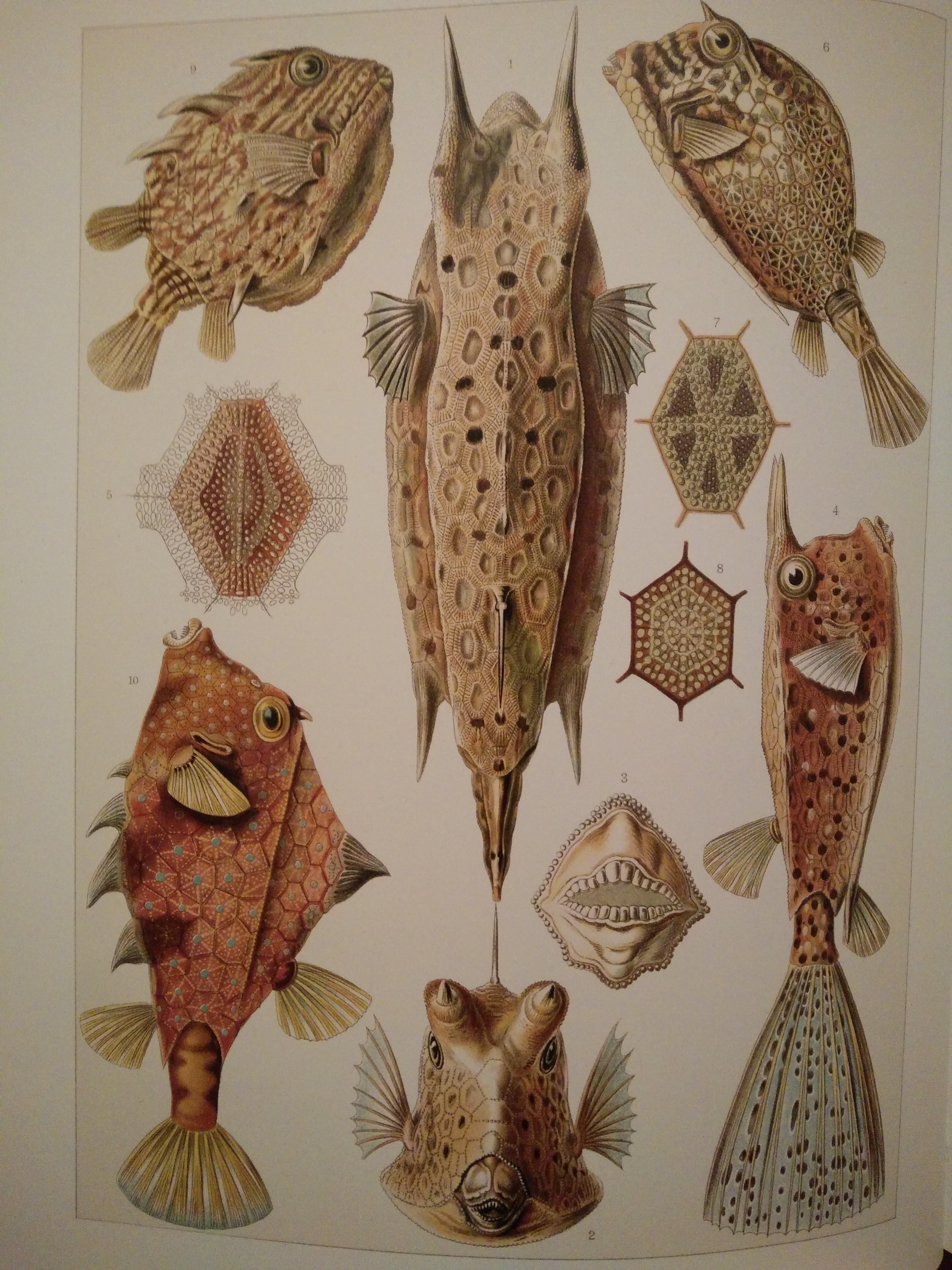
While strolling through my new copy of Ernst Haeckel’s Art Forms in Nature, I noted that one particular creature which Haeckel drew had an almost statement pattern of a Voronoi tessellation on its body. The boxfish’s scales are hexagonal and serrated and act as a body armour for the fish. But because of irregularities on its surface, the scales are non-homogeneous and thus give us a glimpse into nature’s affinity for mathematical beauty. A photo of the relevant page from the book is below.
The graphic at the top of this post: “A Best Effort Voronoi” via VQGAN+CLIP.